Comparison to Biot-Savart

Even though empymod was developed having CSEM in mind, the various inputs make it possible to investigate other acquisition setups such as, for instance, line sources. The simplest way to investigate the magnetic field of line sources is by using the Biot-Savart law for an infinite wire, given by

(1)\[B(r,I) = \frac{\mu_{0} I}{2\pi r} \, ,\]

where \(I\) is the source strength, \(\mu_0\) is the magnetic permeability of free space, and \(r\) is distance.

Let us consider a line source approximated as a very long, but finite bipole with lots of source points, and compare it to the Biot-Savart solution.

Note

This example was contributed by Sil Mossel (@SylvesterOester). You can find out more about his work in his M.Sc. thesis available (from late ‘22 onwards) at the TU Delft Repository.

import empymod
import numpy as np
import matplotlib.pyplot as plt
plt.style.use('ggplot')

Define survey and models

We set the line in the xy-plane at zero depth. The line runs from 0 to 90 metres. This is arbitrary. However, do note that if you would like to investigate the behaviour of the bipole at further distances, the line/bipole should be extended with more source points for it to approximate an infinite wire.

# Source parameters
A = [0, 0, 0.0]      # Start and...
B = [90, 0, 0.0]     # ...end coordinates line
strength = 0.1       # Current I in Ampère. Scalar
freqtime = 83        # Frequency in Hz
srcpts = 401

# Resistivity models
fs_res = [3e8, 3e8]  # Resistivities
hs_res = [3e8, 0.1]  # Resistivities

# Receiver parameters
height = 1           # Heights receivers
nrec = 41            # Number of receivers
rec_posi = [1, 20]   # receivers range from posi 1 to posi 2
recx = np.ones(nrec)*(B[0] - A[0])/2
recy = np.linspace(rec_posi[0], rec_posi[1], nrec)
recz = np.ones(nrec)
rec_y = [recx, recy, recz, 90, 0]
rec_z = [recx, recy, recz, 0, -90]

# Magnetic permeability
mu_0 = 4e-7 * np.pi  # To get from H to B: B = mu0 * H

# Angles and radii
angles = np.arctan(height/rec_y[1])
radii = np.sqrt(height**2 + rec_y[1]**2)

# Different input data for different wires regarding the model:
# fs = fullspace, hs = halfspace
inp = {'src': [A[0], B[0], A[1], B[1], A[2], B[2]], 'depth': [0],
       'freqtime': freqtime, 'srcpts': srcpts, 'mrec': True,
       'strength': strength*mu_0, 'verb': 1}
inp_fs = {'res': fs_res, **inp}
inp_hs = {'res': hs_res, **inp}

Compute empymod

Now we can compute the solutions for the “infinite” wires. Note that to acquire the different components, one should adjust the receiver orientation. The appropriate combinations are:

• (90, 0) = y-dir;

• (0, 0) = x-dir;

• (‘theta’, -90) = z-dir;

(any (‘theta’, -90) is Z as the azimuth does not matter if dip is exactly +/-90; minus sign due to RHS system).

# Compute for different directions
wire_fsy = empymod.bipole(**inp_fs, rec=rec_y)
wire_fsz = empymod.bipole(**inp_fs, rec=rec_z)

wire_hsy = empymod.bipole(**inp_hs, rec=rec_y)
wire_hsz = empymod.bipole(**inp_hs, rec=rec_z)

Calculate Biot-Savart

To investigate the angle between the Biot-Savart and empymod bipole solution, one needs the total field to produce the unit vectors of both solutions.

# Calculate total magnetic fields
wire_tot_fs = np.sqrt(wire_fsy**2 + wire_fsz**2)
wire_tot_hs = np.sqrt(wire_hsy**2 + wire_hsz**2)

# Unit vectors
unitvec_wire_fs = [abs(wire_fsy), abs(wire_fsz)]/abs(wire_tot_fs)
unitvec_wire_hs = [abs(wire_hsy), abs(wire_hsz)]/abs(wire_tot_hs)

# Biot-Savart
Biot_savart_tot = mu_0*strength/(2*np.pi*radii)
Biot_savart_y = np.sin(angles)*Biot_savart_tot
Biot_savart_z = np.cos(angles)*Biot_savart_tot

# Unit vectors Biot-Savart
uv_biot_savart = [Biot_savart_y, Biot_savart_z]/Biot_savart_tot


# Angle difference between Biot-Savart and empymod
def angle_diff(x, y):
    """Angle difference between x and y, in degrees."""
    return np.arccos(np.round(np.sum(x * y, axis=0), 10))*180/np.pi


angle_diff_bs_fs = angle_diff(uv_biot_savart, unitvec_wire_fs)
angle_diff_bs_hs = angle_diff(uv_biot_savart, unitvec_wire_hs)

Plots

Plotting the Biot-Savart and empymod fullspace and halfspace solutions. What is noticeable is that the Biot-Savart and fullspace solution, as well as the Bz-field component from all three solutions, are close to identical. The biggest change is related to the By-component in the halfspace solution. This is related to the relative TE and TM modes. The Bz-field is determined by the TE mode and the By-field to TM. Recalling the reflection coefficients:

(2)\[r_n^{TM} = \frac{\eta_{n+1} \Gamma_{n}-\eta_{n} \Gamma_{n+1}} {\eta_{n+1}\Gamma_{n}+\eta_{n} \Gamma_{n+1}}\, ,\]

(3)\[r_n^{TE} = \frac{\zeta_{n+1} \Gamma_{n}-\zeta_{n} \Gamma_{n+1}} {\zeta_{n+1} \Gamma_{n}+\zeta_{n} \Gamma_{n+1}}\, .\]

Since the conductivity of air almost zero, in a half-space the local reflection coefficient \(r^{TM} = 1\). At the same time, \(r^{TE}\) is dominated by \(\mu_0\) which is similar in air as in any soil, making the reflection coefficient for the TE mode equal to zero.

# Plot total fields.
fig, ((ax1, ax2), (ax3, ax4)) = plt.subplots(
        2, 2, figsize=(8, 6), sharex=True, constrained_layout=True)

ax1.set_title('Bz-field away from cable')
ax1.set_ylabel('Amplitude (nT)')
ax1.plot(radii, abs(wire_fsz) * 1e9, 'C3+-', label='Wire FS')
ax1.plot(radii, abs(wire_hsz) * 1e9, 'C5x-', label='Wire HS')
ax1.plot(radii, abs(Biot_savart_z) * 1e9, 'C1.-', label='Biot-Savart')
ax1.set_ylim([0, 15])
ax1.legend()

ax2.set_title('By-field')
ax2.set_ylabel('Amplitude (nT)')
ax2.plot(radii, abs(wire_fsy) * 1e9, 'C3+-', label='Wire FS')
ax2.plot(radii, abs(wire_hsy) * 1e9, 'C5x-', label='Wire HS')
ax2.plot(radii, abs(Biot_savart_y) * 1e9, 'C1.-', label='Biot-Savart')
ax2.set_ylim([0, 15])
ax2.legend()

ax3.set_title('Total B-field away from cable')
ax3.set_xlabel('Receiver distance (m)')
ax3.set_ylabel('Amplitude (nT)')
ax3.plot(radii, abs(wire_tot_fs) * 1e9, 'C3+-', label='Wire FS')
ax3.plot(radii, abs(wire_tot_hs) * 1e9, 'C5x-', label='Wire HS')
ax3.plot(radii, abs(Biot_savart_tot) * 1e9, 'C1.-', label='Biot-Savart')
ax3.set_ylim([0, 15])
ax3.legend()

ax4.set_title('Angle diff. Biot-Savart and HS-sol.')
ax4.set_xlabel('Receiver distance (m)')
ax4.set_ylabel('Angle (degrees)')
ax4.plot(radii, abs(angle_diff_bs_hs), 'C3+-')
plt.show()

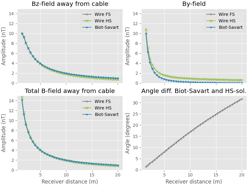
The total field and By and Bz components are compared. The bottom right shows the angle difference between the vectors of the Biot-Savart and bipole half-space solution.

If we take a finite length wire, eventually Biot-Savart for an infinite length wire will not apply. The question is: at what receiver distance relative to the finite wire is Biot-Savart still decently applicable. When testing this in empymod and comparing Biot-Savart for an infinite line source to a finite length wire, it is has been concluded that when the receiver is a 1/10th of the length of the wire away from its middle, Biot-Savart and empymod agree within 2%. For 1% accuracy between the two methods, the receiver distance should not extend more than 7% of the length of the wire.

empymod.Report()

Sun Oct 16 11:49:50 2022 UTC
OS	Linux	CPU(s)	2	Machine	x86_64
Architecture	64bit	RAM	7.6 GiB	Environment	Python
File system	ext4
Python 3.8.6 (default, Oct 19 2020, 15:10:29) [GCC 7.5.0]
numpy	1.23.4	scipy	1.9.2	numba	0.56.3
empymod	2.2.2.dev5+gecfe950	IPython	8.5.0	matplotlib	3.6.1

Estimated memory usage: 11 MB